02 Prepare : k-Nearest Neighbors
Reading
Before coming to class this week, please study the following:
Machine Learning, Section 2.1 Some Terminology
Machine Learning, Section 2.2 Knowing What You Know
Machine Learning, Section 7.2 Nearest Neighbour Methods
k-Nearest Neighbors Algorithm
k-Nearest Neighbors is a simple classification algorithm.
Visualizing the Data
To understand how the algorithm works, let's look at a graph showing part of the Iris dataset samples plotted using two of their features, petal length and petal width:
(If you've forgotten the details of the Iris dataset, please review them here before continuing.)
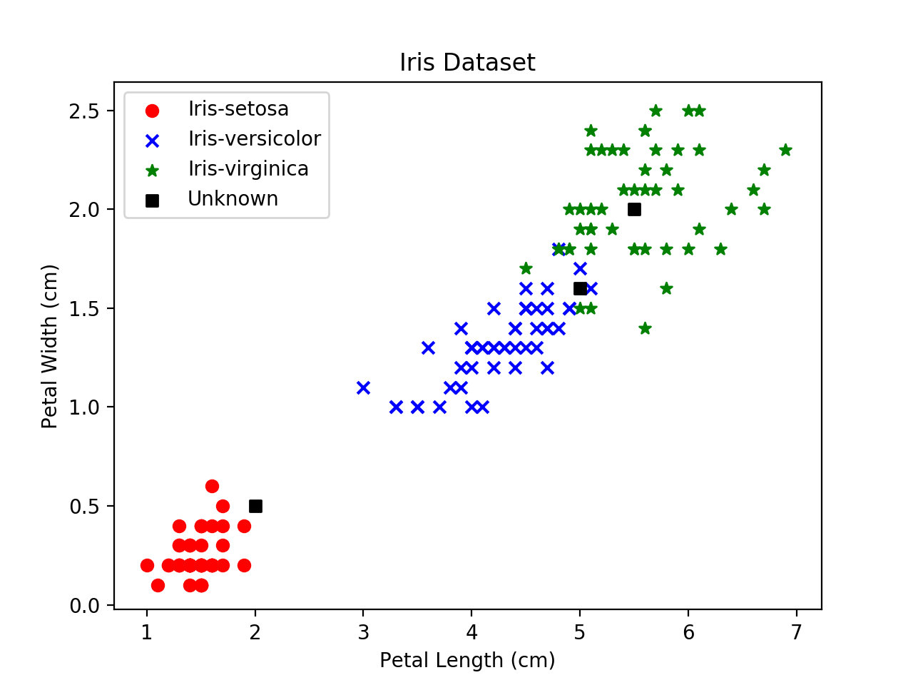
Each colored point on the plot represents one sample from the "training data".
The three black squares represent samples from the test data, whose species we want the algorithm to classify.
The Algorithm
The k-Nearest Neighbors algorithm allows us to predict which class a new sample belongs to by following these steps:
Choose a value for k.
For each sample, $x_i$, in the training data:
Find the k "closest" points to $x_i$.
Tally up how many times each class occurs within those k points.
Sample $x_i$ is predicted to belong to the class which has the most occurrances.
Example
Below is a zoomed-in view of one of the unknown samples. Let's imagine we choose to make k=3. The purple circle shows the 3 samples from the training data that are closest to the unknown sample.[1]
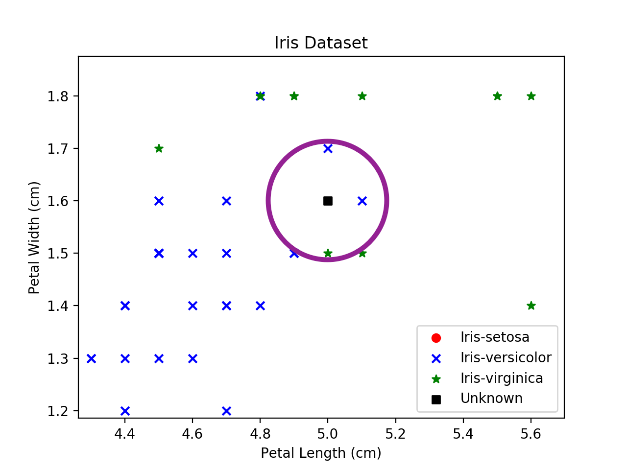
Since there are two samples belonging to the Iris versicolor class and only belonging to Iris virginica, the algorithm predicts that the unknown sample is an Iris versicolor.
Assumptions & Considerations
Every machine learning algorithm comes with some assumptions about the data it's processing. It's important to understand those assumptions, otherwise the predictions the algorithm makes won't be useful.
Measuring Distance
A major assumption made by k-NN is that there is some meaningful way to measure the distance between the samples. There are several ways to calculate the distance between neighbors. The most common method is to use Euclidean Distance. For 2-dimensional data, this can be calculated as:
$$ distance = \sqrt{(x_2 - x_1)^2 + (y_2 - y_1)^2} $$
For m-dimensional data, this generalizes to:
$$ distance = \sqrt{(x_2 - x_1)^2 + (y_2 - y_1)^2 + ... + (m_2 - m_1)^2} $$
There are many other ways to measure the distance between two samples, including Manhattan distance and Chebyshev distance metrics. (All three of the above are specific versions of another metric you'll often see discussed, called the Minkowski distance metric.
Custom Metrics
Aside from those mentioned above, any metric can be used to measure the distance between samples, so long as it meets the following four criteria:[2]
-
The distance between any two samples is not a negative number. (non-negativity or separation axiom)
-
The distance between any sample and itself is 0. (identity of indiscernibles)
-
The distance between any two points, $a$ and $b$ is the same as the distance between point $b$ and $a$. (symmetry)
-
It doesn't result in a violation of the Triangle Inequality Theorem (subadditivity).
Unfortunately, there isn't an easy way to say which metric would be the "best".
We could test them all on a given set of training and test data and determine which performs the best, but each metric comes with its own assumptions about what the distance between samples represents.
Often, you'll need to think about the specific type of data, and the features under consideration in order to choose the most reasonable metric for your situation.
Scaling/Normalizing the data
In many cases, we'll need to scale or normalize the data before processing. (A process that is sometimes referred to as "pre-processing")
Imagine you're trying to use your kNN classifier to classify people into potential customers for a product. You survey a bunch of customers and use the features of age and annual salary:
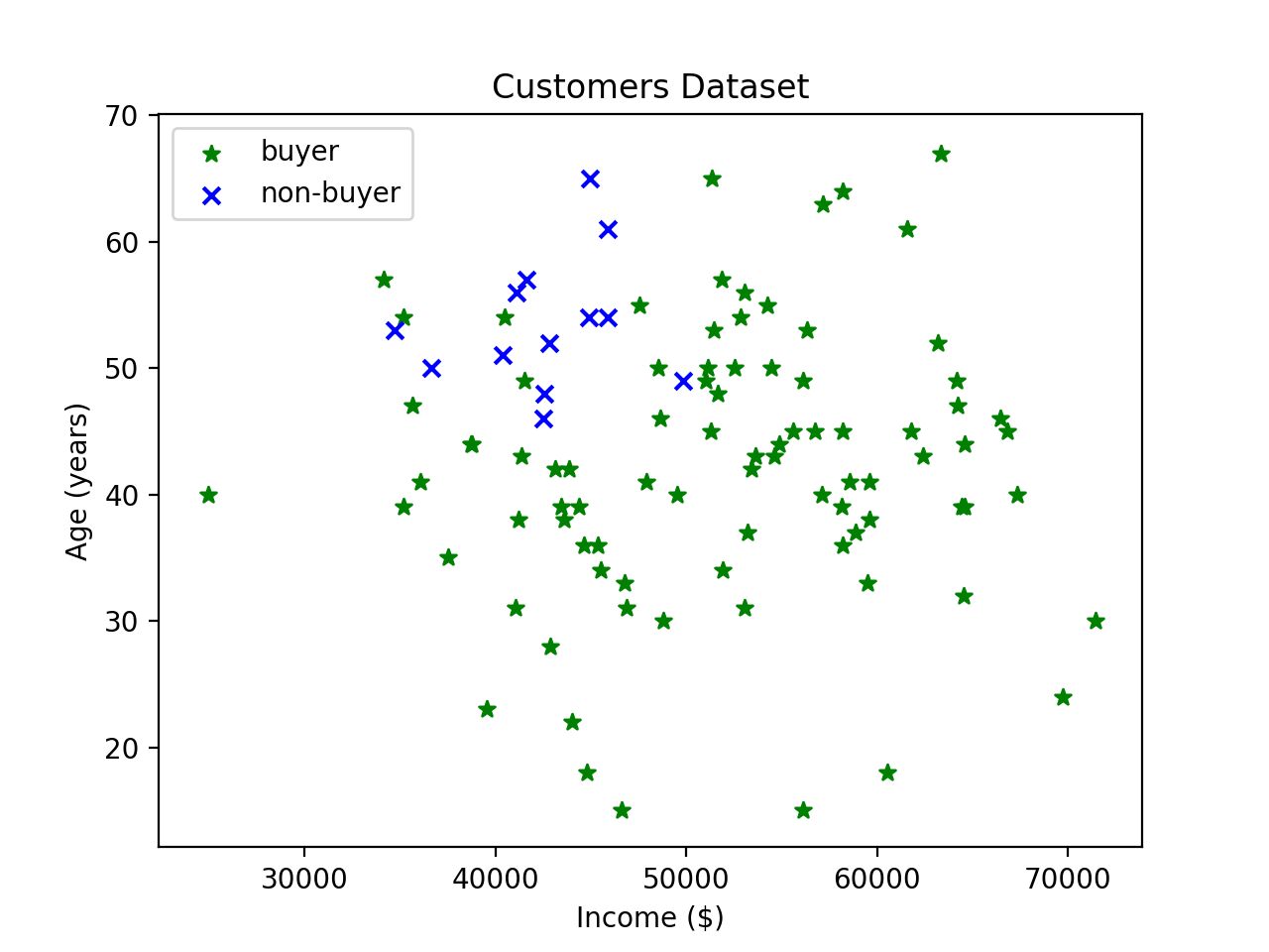
Consider two incomes that differ by 10% compared to two ages that differ by 10%:
$$ distance = \sqrt{(55000 - 50000)^2 + (33 - 30)^2} $$
Because incomes are several orders of magnitude greater than ages, the income feature will have a much stronger effect on the classification than the age feature.
To solve this, we can scale or normalize the data. There are two common approaches to this. First, you can do what's called min-max scaling (sometimes also called normalization) on each value:
$$ x' = \frac{x - x_{min}}{x_{max} - x_{min}} $$
This causes every value to rescale to fit within the range of 0 to 1. (the previous lowest value will become 0, and the previous highest value will become 1, everything else will fall between those values).
For kNN however, a more robust approach is to use Z-score normalization (sometimes also called standardization):
$$ x' = \frac{x - \mu}{\sigma} $$
Where, $\mu$ is the mean of the feature being transformed, and $\sigma$ is its standard deviation.
If we standardize the income and age data, notice how the scale changes without affecting the relative positions of the samples:
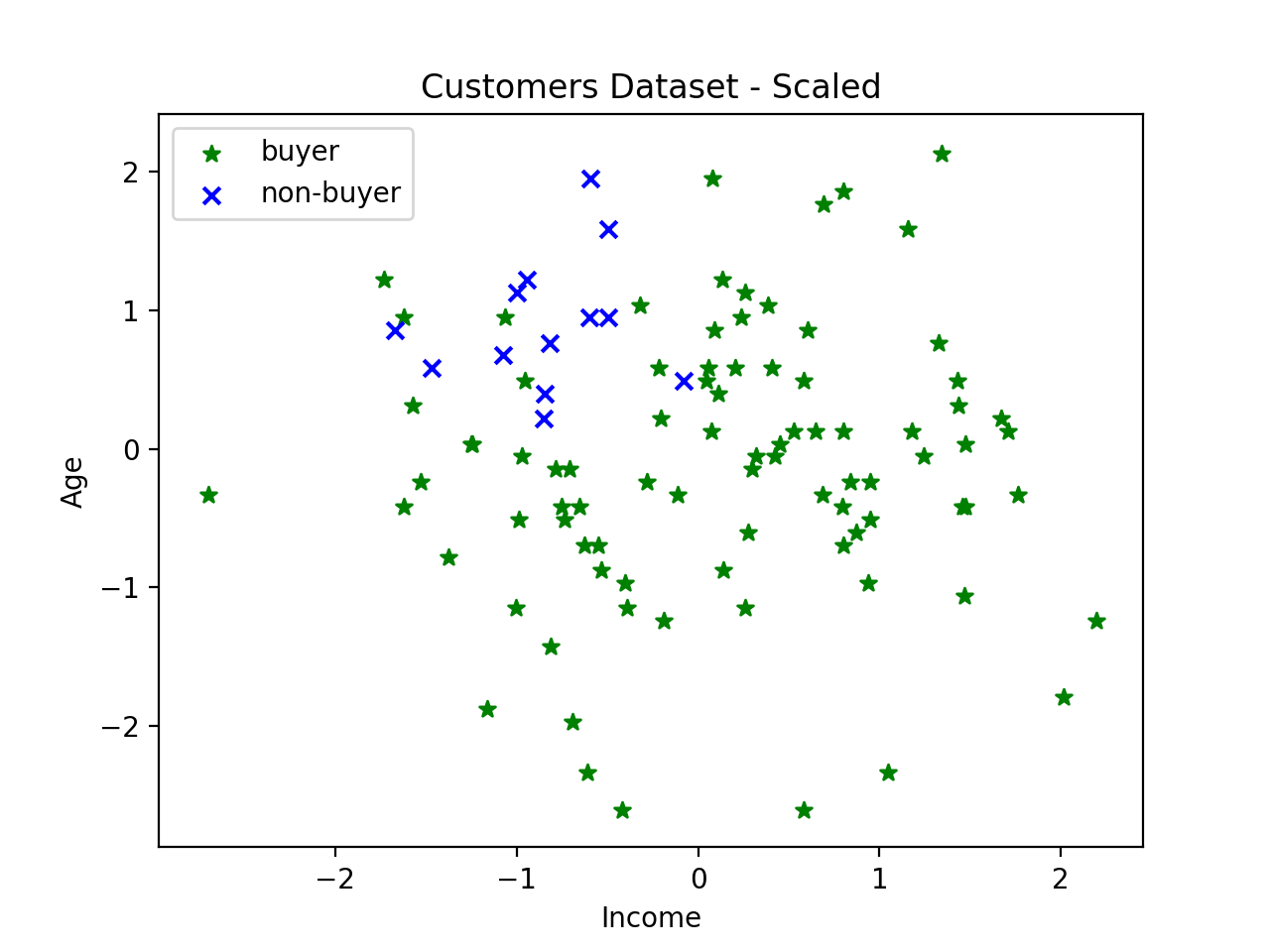
Since both features now use the same scale, they will have equal weight when calculating the distance between points.
WarningYou should be aware that many books and articles use the terms "normalization", "scaling", and "standardization" interchangeably. The way we've used the terms above is how they are most commonly used in statistics, but even amongst statisticians there can be some disagreement.[3]
When reading a description of pre-processing, it's important to understand exactly what kind of transformation the author is describing, regardless of what terminology they use.
Choosing k
Another issue to consider in kNN is what value to choose for k. If the value is too large, samples that are very distant may have an undue influence on the classification.
If the value is too small, the algorithm will be too sensitive to the influence of each sample.
Unfortunately, there is no best answer for how to choose k, but there are some guidelines you can follow to figure out the best value for your specific dataset:
-
The value for
kshould not be an even number, as this can result in ties when counting which class is most common amongst the nearest neighbors. -
The value for
kshould not be a multiple of the number of classes, for the same reason as above. (So choosing 3, 6, 9, etc... for the iris dataset would potentially result in a tie because there are 3 classes in the data. -
A good starting point for
kis the square root of the number of samples in your dataset. -
You should run the algorithm multiple times with different values of
kand compare the results.
Seeing it in action
You can see the algorithm in action and play around with the points with this interactive site.
References
1. Closest in terms of Euclidean Distance. See part 2 for a discussion of distance measurements.↩
2. See the definition of a Metric for a more detailed discussion.↩
3. See this article for a more detailed discussion of normalization and scaling.↩